Accuracy
Contents
2.5. Accuracy#
In a census, the access frame matches the population, and the sample captures the entire population. In this situation, if we administer a well-designed questionnaire, then we have complete and accurate information on the population, and the scope is perfect. Similarly in measuring CO2 concentrations in the atmosphere, if our instrument has perfect accuracy and is properly used, then we can measure the exact value of the CO2 concentration (ignoring air fluctuations). These situations are rare, if not impossible. In most settings, we need to quantify the accuracy of our measurements in order to generalize our findings to the unobserved. For example, we often use the sample to estimate an average value for a population, infer the value of a scientific unknown from measurements, or predict the behavior of a new individual. In each of these settings, we also want a quantifiable degree of accuracy. We want to know how close our estimates, inferences, and predictions are to the truth.
The analogy of darts thrown at a dart board that was introduced earlier can be useful in understanding accuracy. We divide accuracy into two basic parts: bias and precision (also known as variation). Our goal is for the darts to hit the bullseye on the dart board and for the bullseye to line up with the unseen target. The spray of the darts on the board represents the precision in our measurements, and the gap from the bullseye to the unknown value that we are targeting represents the bias.
Figure 2.5 shows combinations of low and high bias and precision. In each of these diagrams, the dots represent the measurements taken, and the star represents the true, unknown parameter value. The dots form a scattershot within the access frame represented by the dart board. When the bullseye of the access frame is roughly centered on the star (top row), the measurements are scattered around the value of interest and bias is low. The larger dart boards (right column) indicate a wider spread (lower precision) in the measurements.
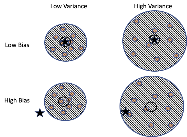
Fig. 2.5 Combinations of low and high measurement bias and precision#
Representative data puts us in the top row of the diagram, where there is low bias, meaning that the unknown target aligns with the bullseye. Ideally, our instruments and protocols put us in the upper-left part of the diagram, where the variation is also low. The pattern of points in the bottom row systematically misses the targeted value. Taking larger samples will not correct this bias.
2.5.1. Types of Bias#
Bias comes in many forms. We describe some classic types here and connect them to our target-access-sample framework.
- Coverage bias
Occurs when the access frame does not include everyone in the target population. For example, a survey based on phone calls cannot reach those without a phone. In this situation, those who cannot be reached may differ in important ways from those in the access frame.
- Selection bias
Arises when the mechanism used to choose units for the sample tends to select certain units more often than they should be selected. As an example, a convenience sample chooses the units that are most easily available. Problems can arise when those who are easy to reach differ in important ways from those who are harder to reach. As another example, observational studies and experiments often rely on volunteers (people who choose to participate), and this self-selection has the potential for bias if the volunteers differ from the target population in important ways.
- Nonresponse bias
Comes in two forms: unit and item. Unit nonresponse happens when someone selected for a sample is unwilling to participate (they may never answer a phone call from an unknown caller). Item nonresponse occurs when, say, someone answers the phone but refuses to respond to a particular survey question. Nonresponse can lead to bias if those who choose not to respond are systematically different from those who choose to respond.
- Measurement bias
Happens when an instrument systematically misses the target in one direction. For example, low humidity can systematically give us incorrectly high measurements of air pollution. In addition, measurement devices can become unstable and drift over time and so produce systematic errors. In surveys, measurement bias can arise when questions are confusingly worded or leading, or when respondents may not be comfortable answering honestly.
Each of these types of bias can lead to situations where the data are not centered on the unknown targeted value. Often, we cannot assess the potential magnitude of the bias, since little to no information is available on those who are outside the access frame, less likely to be selected for the sample, or disinclined to respond. Protocols are key to reducing these sources of bias. Chance mechanisms to select a sample from the frame or to assign units to experimental conditions can eliminate selection bias. A nonresponse follow-up protocol to encourage participation can reduce nonresponse bias. A pilot survey can improve question wording and so reduce measurement bias. Procedures to calibrate instruments and protocols to take measurements in, say, random order can reduce measurement bias.
In the 2016 US presidential election, nonresponse bias and measurement bias were key factors in the inaccurate predictions of the winner. Nearly all voter polls leading up to the election predicted Clinton a winner over Trump. Trump’s upset victory came as a surprise. After the election, many polling experts attempted to diagnose where things went wrong in the polls. The American Association for Public Opinion Research found that the predictions were flawed for two key reasons:
College-educated voters were overrepresented. College-educated voters are more likely to participate in surveys than those with less education, and in 2016 they were more likely to support Clinton. Higher response rates from more highly educated voters biased the sample and overestimated support for Clinton.
Voters were undecided or changed their preferences a few days before the election. Since a poll is static and can only directly measure current beliefs, it cannot reflect a shift in attitudes.
It’s difficult to figure out whether people held back their preference or changed their preference and how large a bias this created. However, exit polls have helped polling experts understand what happened after the fact. They indicate that in battleground states, such as Michigan, many voters made their choice in the final week of the campaign, and that group went for Trump by a wide margin.
Bias does not need to be avoided under all circumstances. If an instrument is highly precise (low variance) and has a small bias, then that instrument might be preferable to another with higher variance and no bias. As an example, biased studies are potentially useful to pilot a survey instrument or to capture useful information for the design of a larger study. Many times we can at best recruit volunteers for a study. Given this limitation, it can still be useful to enroll these volunteers in the study and use random assignment to split them into treatment groups. That’s the idea behind randomized controlled experiments.
Whether or not bias is present, data typically also exhibit variation. Variation can be introduced purposely by using a chance mechanism to select a sample, and it can occur naturally through an instrument’s precision. In the next section, we identify three common sources of variation.
2.5.2. Types of Variation#
The following types of variation results from a chance mechanism and have the advantage of being quantifiable:
- Sampling variation
Results from using chance to select a sample. In this case, we can, in principle, compute the chance that a particular collection of elements is selected for the sample.
- Assignment variation
Occurs in a controlled experiment when we assign units at random to treatment groups. In this situation, if we split the units up differently, then we can get different results from the experiment. This assignment process allows us to compute the chance of a particular group assignment.
- Measurement error
Results from the measurement process. If the instrument used for measurement has no drift or bias and a reliable distribution of errors, then when we take multiple measurements on the same object, we get random variations in measurements that are centered on the truth.
The urn model is a simple abstraction that can be helpful for understanding variation. This model sets up a container (an urn, which is like a vase or a bucket) full of identical marbles that have been labeled, and we use the simple action of drawing marbles from the urn to reason about sampling schemes, randomized controlled experiments, and measurement error. For each of these types of variation, the urn model helps us estimate the size of the variation using either probability or simulation (see Chapter 3). The example of selecting Wikipedia contributors to receive an informal award provides two examples of the urn model.
Recall that for the Wikipedia experiment, 200 contributors were selected at random from 1,440 top contributors. These 200 contributors were then split, again at random, into two groups of 100 each. One group received an informal award and the other didn’t. Here’s how we use the urn model to characterize this process of selection and splitting:
Imagine an urn filled with 1,440 marbles that are identical in shape and size, and written on each marble is one of the 1,440 Wikipedia usernames. (This is the access frame.)
Mix the marbles in the urn really well, select one marble, and set it aside.
Repeat the mixing and selecting of the marbles to obtain 200 marbles.
The marbles drawn form the sample. Next, to determine which of the 200 contributors receive awards, we work with another urn:
In a second urn, put in the 200 marbles from the preceding sample.
Mix these marbles well, select one marble, and set it aside.
Repeat, choosing 100 marbles. That is, choose marbles one at a time, mixing in between, and setting the chosen marble aside.
The 100 drawn marbles are assigned to the treatment group and correspond to the contributors who receive an award. The 100 left in the urn form the control group and receive no award.
Both the selection of the sample and the choice of award recipients use a chance mechanism. If we were to repeat the first sampling activity again, returning all 1,440 marbles to the original urn, then we would most likely get a different sample. This variation is the source of sampling variation. Likewise, if we were to repeat the random assignment process again (keeping the sample of 200 unchanged), then we would get a different treatment group. Assignment variation arises from this second chance process.
The Wikipedia experiment provided an example of both sampling and assignment variation. In both cases, the researcher imposed a chance mechanism on the data collection process. Measurement error can at times also be considered a chance process that follows an urn model. For example, we can characterize the measurement error of the CO2 monitor at Mauna Loa in this way.
If we can draw an accurate analogy between variation in the data and the urn model, the urn model provides us the tools to estimate the size of the variation (see Chapter 3). This is highly desirable because we can give concrete values for the variation in our data. However, it’s vital to confirm that the urn model is a reasonable depiction of the source of variation. Otherwise, our claims of accuracy can be seriously flawed. Knowing as much as possible about data scope, including instruments and protocols and chance mechanisms used in data collection, is needed to apply these urn models.