The Urn Model
Contents
3.1. The Urn Model#
The urn model was developed by Jacob Bernoulli in the early 1700s as a way to model the process of selecting items from a population. The urn model shown in Figure 3.1 gives a visual description of the process of randomly sampling marbles from an urn. Five marbles were originally in the urn: three black and two white. The diagram shows that two draws were made; first a white marble was drawn and then a black marble.
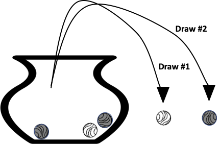
Fig. 3.1 Diagram of two marbles being drawn, without replacement, from an urn#
To set up an urn model, we first need to make a few decisions:
The number of marbles in the urn
The color (or label) on each marble
The number of marbles to draw from the urn
Finally, we also need to decide the sampling process. For our process, we mix the marbles in the urn, and as we select a marble for our sample, we can choose to record the color and return the marble to the urn (with replacement), or set aside the marble so that it cannot be drawn again (without replacement).
These decisions make up the parameters of our model. We can adapt the urn model to describe many real-world situations by our choice for these parameters. To illustrate, consider the example in Figure 3.1. We can simulate the draw of two marbles from our urn without replacement between draws using numpy’s random.choice method. The numpy library supports functions for arrays, which can be particularly useful for data science:
import numpy as np

urn = ["b", "b", "b", "w", "w"]
print("Sample 1:", np.random.choice(urn, size=2, replace=False))
print("Sample 2:", np.random.choice(urn, size=2, replace=False))
Sample 1: ['b' 'w']
Sample 2: ['w' 'b']
Notice that we set the replace argument to False to indicate that once we sample a marble, we don’t return it to the urn.
With this basic setup, we can get approximate answers to questions about the kinds of samples we would expect to see. What is the chance that our sample contains marbles of only one color? Does the chance change if we return each marble after selecting it? What if we changed the number of marbles in the urn? What if we draw more marbles from the urn? What happens if we repeat the process many times?
The answers to these questions are fundamental to our understanding of data collection. We can build from these basic skills to simulate the urn and apply simulation techniques to real-world problems that can’t be easily solved with classic probability equations.
For example, we can use simulation to easily estimate the fraction of samples where both marbles that we draw match in color. In the following code, we run 10,000 rounds of sampling two marbles from our urn. Using these samples, we can directly compute the proportion of samples with matching marbles:
n = 10_000
samples = [np.random.choice(urn, size=2, replace=False) for _ in range(n)]
is_matching = [marble1 == marble2 for marble1, marble2 in samples]
print(f"Proportion of samples with matching marbles: {np.mean(is_matching)}")
Proportion of samples with matching marbles: 0.4032
We just carried out a simulation study. Our call to np.random.choice imitates the chance process of drawing two marbles from the urn without replacement. Each call to np.random.choice gives us one possible sample. In a simulation study, we repeat this chance process many times (10_000 in this case) to get a whole bunch of samples. Then we use the typical behavior of these samples to reason about what we might expect to get from the chance process. While this might seem like a contrived example (it is), consider if we replaced the marbles with people on a dating service, replaced the colors with more complex attributes, and perhaps used a neural network to score a match and you can start to see the foundation of much more sophisticated analysis.
So far we have focused on the sample, but we are often interested in the relationship between the sample we might observe and what it can tell us about the “population” of marbles that were originally in the urn.
We can draw an analogy to data scope from Chapter 2: a set of marbles drawn from the urn is a sample, and the collection of all marbles placed in the urn is the access frame, which in this situation we take to be the same as the population. This blurring of the difference between the access frame and the population points to the gap between simulation and reality. Simulations tend to simplify models. Nonetheless, they can give helpful insights to real-world phenomena.
The urn model, where we do not replace the marbles between draws, is a common selection method called the simple random sample. We describe this method and other sampling techniques based on it next.
3.1.1. Sampling Designs#
The process of drawing marbles without replacement from an urn is equivalent to a simple random sample. In a simple random sample, every sample has the same chance of being selected. While the method name has the word simple in it, constructing a simple random sample is often anything, but simple and in many cases is also the best sampling procedure. Plus, if we are being honest, it can also be a little confusing.
To better understand this sampling method we return to the urn model. Consider an urn with seven marbles. Instead of coloring the marbles, we label each uniquely with a letter A through G. Since each marble has a different label, we can more clearly identify all possible samples that we might get. Let’s select three marbles from the urn without replacement, and use the itertools library to generate the list of all combinations:
from itertools import combinations

all_samples = ["".join(sample) for sample in combinations("ABCDEFG", 3)]
print(all_samples)
print("Number of Samples:", len(all_samples))
['ABC', 'ABD', 'ABE', 'ABF', 'ABG', 'ACD', 'ACE', 'ACF', 'ACG', 'ADE', 'ADF', 'ADG', 'AEF', 'AEG', 'AFG', 'BCD', 'BCE', 'BCF', 'BCG', 'BDE', 'BDF', 'BDG', 'BEF', 'BEG', 'BFG', 'CDE', 'CDF', 'CDG', 'CEF', 'CEG', 'CFG', 'DEF', 'DEG', 'DFG', 'EFG']
Number of Samples: 35
Our list shows that there are 35 unique sets of three marbles. We could have drawn each of these sets six different ways. For example, the set \(\{A, B, C\}\) can be sampled:
from itertools import permutations

print(["".join(sample) for sample in permutations("ABC")])
['ABC', 'ACB', 'BAC', 'BCA', 'CAB', 'CBA']
In this small example, we can get a complete picture of all the ways in which we can draw any three marbles from the urn.
Since each set of three marbles from the population of seven is equally likely to occur, the chance of any one particular sample must be \(1/35\):
We use the special symbol \({\mathbb{P}}\) to stand for “probability” or “chance,” and we read the statement \({\mathbb{P}}(ABC)\) as “the chance the sample contains the marbles labeled A, B, and C in any order.”
We can use the enumeration of all of the possible samples from the urn to answer additional questions about this chance process. For example, to find the chance that marble \(A\) is in the sample, we can add up the chance of all samples that contain \(A\). There are 15 of them, so the chance is:
When it’s too difficult to list and count all of the possible samples, we can use simulation to help understand this chance process.
Note
Many people mistakenly think that the defining property of a simple random sample is that every unit has an equal chance of being in the sample. However, this is not the case. A simple random sample of \(n\) units from a population of \(N\) means that every possible collection of \(n\) of the \(N\) units has the same chance of being selected. A slight variant of this is the simple random sample with replacement, where the units/marbles are returned to the urn after each draw. This method also has the property that every sample of \(n\) units from a population of \(N\) is equally likely to be selected. The difference, though, is that there are more possible sets of \(n\) units because the same marble can appear more than once in the sample.
The simple random sample (and its corresponding urn) is the main building block for more complex survey designs. We briefly describe two of the more widely used designs:
- Stratified sampling
Divide the population into nonoverlapping groups, called strata (one group is called a stratum and more than one are strata), and then take a simple random sample from each. This is like having a separate urn for each stratum and drawing marbles from each urn, independently. The strata do not have to be the same size, and we need not take the same number of marbles from each.
- Cluster sampling
Divide the population into nonoverlapping subgroups, called clusters, take a simple random sample of the clusters, and include all of the units in a cluster in the sample. We can think of this as a simple random sample from one urn that contains large marbles that are themselves containers of small marbles. (The large marbles need not have the same number of marbles in them.) When opened, the sample of large marbles turns into the sample of small marbles. (Clusters tend to be smaller than strata.)
As an example, we might organize our seven marbles, labeled \(A\)–\(G\), into three clusters, \((A, B)\), \((C,D)\), and \((E, F, G)\). Then, a cluster sample of size one has an equal chance of drawing any of the three clusters. In this scenario, each marble has the same chance of being in the sample:
But every combination of elements is not equally likely: it is not possible for the sample to include both \(A\) and \(C\), because they are in different clusters.
Often, we are interested in a summary of the sample; in other words, we are interested in a statistic. For any sample, we can calculate the statistic, and the urn model helps us find the distribution of possible values that statistic may take on. Next, we examine the distribution of a statistic for our simple example.
3.1.2. Sampling Distribution of a Statistic#
Suppose we are interested in testing the failure pressure of a new fuel tank design for a rocket. It’s expensive to carry out the pressure tests since we need to destroy the fuel tank, and we may need to test more than one fuel tank to address variations in manufacturing.
We can use the urn model to choose the prototypes to be tested, and we can summarize our test results by the proportion of prototypes that fail the test. The urn model provides us the knowledge that each of the samples has the same chance of being selected, and so the pressure test results are representative of the population.
To keep the example simple, let’s say we have seven fuel tanks that are labeled like the marbles from before. Let’s see what happens when tanks \(A\), \(B\), \(D\), and \(F\) fail the pressure test, if chosen, and tanks \(C\), \(E\), and \(G\) pass.
For each sample of three marbles, we can find the proportion of failures according to how many of these four defective prototypes are in the sample. We give a few examples of this calculation:
Sample |
ABC |
BCE |
BDF |
CEG |
|---|---|---|---|---|
Proportion |
2/3 |
1/3 |
1 |
0 |
Since we are drawing three marbles from the urn, the only possible sample proportions are \(0\), \(1/3\), \(2/3\), and \(1\), and for each triple, we can calculate its corresponding proportion. There are four samples that give us all failed tests (a sample proportion of 1). These are \(ABD\), \(ABF\), \(ADF\), and \(BDF\), so the chance of observing a sample proportion of 1 is \(4/35\). We can summarize the distribution of values for the sample proportion into a table, which we call the sampling distribution of the proportion:
Proportion of failures |
No. of samples |
Fraction of samples |
|---|---|---|
0 |
1 |
1/35 \(\approx 0.03\) |
1/3 |
12 |
12/35 \(\approx 0.34\) |
2/3 |
18 |
18/35 \(\approx 0.51\) |
1 |
4 |
4/35 \(\approx 0.11\) |
Total |
35 |
1 |
While these calculations are relatively straightforward, we can approximate them through a simulation study. To do this, we take samples of three from our population over and over—say 10,000 times. For each sample, we calculate the proportion of failures. That gives us 10,000 simulated sample proportions. The table of the simulated proportions should come close to the sampling distribution. We confirm this with a simulation study.
3.1.3. Simulating the Sampling Distribution#
Simulation can be a powerful tool to understand complex random processes. In our example of seven fuel tanks, we are able to consider all possible samples from the corresponding urn model. However, in situations with large populations and samples and more complex sampling processes, it may not be tractable to directly compute the chance of certain outcomes. In these situations, we often turn to simulation to provide accurate estimates of the quantities we can’t compute directly.
Let’s set up the problem of finding the sampling distribution of the proportion of failures in a simple random sample of three fuel tanks as an urn model. Since we are interested in whether or not the tank fails, we use 1 to indicate a failure and 0 to indicate a pass, giving us an urn with marbles labeled as follows:
urn = [1, 1, 0, 1, 0, 1, 0]
We have encoded the tanks \(A\) through \(G\) using 1 for fail and 0 for pass, so we can take the mean of the sample to get the proportion of failures in a sample:
sample = np.random.choice(urn, size=3, replace=False)
print(f"Sample: {sample}")
print(f"Prop Failures: {sample.mean()}")
Sample: [1 0 0]
Prop Failures: 0.3333333333333333
In a simulation study, we repeat the sampling process thousands of times to get thousands of proportions, and then we estimate the sampling distribution of the proportion from what we get in our simulation. Here, we construct 10,000 samples (and so 10,000 proportions):
samples = [np.random.choice(urn, size=3, replace=False) for _ in range(10_000)]
prop_failures = [s.mean() for s in samples]
We can study these 10,000 sample proportions and match our findings against what we calculated already using the complete enumeration of all 35 possible samples. We expect the simulation results to be close to our earlier calculations because we have repeated the sampling process many, many times. That is, we want to compare the fraction of the 10,000-sample proportion that is 0, \(1/3\), \(2/3\), and 1 to those we computed exactly; those fractions are \(1/35\), \(12/35\), \(18/35\), and \(4/35\), or about \(0.03\), \(0.34\), \(0.51\), and \(0.11\):
unique_els, counts_els = np.unique(prop_failures, return_counts=True)
pd.DataFrame({
    "Proportion of failures": unique_els,
    "Fraction of samples": counts_els / 10_000,
})
| Proportion of Failures | Fraction of Samples | |
|---|---|---|
| 0 | 0.00 | 0.03 |
| 1 | 0.33 | 0.35 |
| 2 | 0.67 | 0.51 |
| 3 | 1.00 | 0.11 |
The simulation results closely match the exact chances that we calculated earlier.
Note
Simulation studies leverage random number generators to sample many outcomes from a random process. In a sense, simulation studies convert complex random processes into data that we can readily analyze using the broad set of computational tools we cover in this book. While simulation studies typically do not provide definitive proof of a particular hypothesis, they can provide important evidence. In many situations, simulation is the most accurate estimation process we have.
Drawing marbles from an urn with 0s and 1s is such a popular framework for understanding randomness that this chance process has been given a formal name, hypergeometric distribution, and most software provides functionality to rapidly carry out simulations of this process. In the next section, we simulate the hypergeometric distribution of the fuel tank example.
3.1.4. Simulation with the Hypergeometric Distribution#
Instead of using random.choice, we can use numpy’s random.hypergeometric to simulate drawing marbles from the urn and counting the number of failures. The random.hypergeometric method is optimized for the 0-1 urn and allows us to ask for 10,000 simulations in one call. For completeness, we repeat our simulation study and calculate the empirical proportions:
simulations_fast = np.random.hypergeometric(
    ngood=4, nbad=3, nsample=3, size=10_000
)
print(simulations_fast)
[1 1 2 ... 1 2 2]
(We don’t think that a pass is “bad”; it’s just a naming convention to call the type you want to count “good” and the other “bad”.)
We tally the fraction of the 10,000 samples with 0, 1, 2, or 3 failures:
unique_els, counts_els = np.unique(simulations_fast, return_counts=True)
pd.DataFrame({
    "Number of failures": unique_els,
    "Fraction of samples": counts_els / 10_000,
})
| Number of Failures | Fraction of Samples | |
|---|---|---|
| 0 | 0 | 0.03 |
| 1 | 1 | 0.34 |
| 2 | 2 | 0.52 |
| 3 | 3 | 0.11 |
You might have asked yourself already: since the hypergeometric is so popular, why not provide the exact distribution of the possible values? In fact, we can calculate these exactly:
from scipy.stats import hypergeom

num_failures = [0, 1, 2, 3]
pd.DataFrame({
    "Number of failures": num_failures,
    "Fraction of samples": hypergeom.pmf(num_failures, 7, 4, 3),
})
| Number of Failures | Fraction of Samples | |
|---|---|---|
| 0 | 0 | 0.03 |
| 1 | 1 | 0.34 |
| 2 | 2 | 0.51 |
| 3 | 3 | 0.11 |
Note
Whenever possible, it’s a good idea to use the functionality provided in a third-party package for simulating from a named distribution, such as the random number generators offered in numpy, rather than writing your own function. It’s best to take advantage of efficient and accurate code that others have developed. That said, building from scratch on occasion can help you gain an understanding of an algorithm, so we recommend trying it.
Perhaps the two most common chance processes are those that arise from counting the number of 1s drawn from a 0-1 urn: drawing without replacement is the hypergeometric distribution and drawing with replacement is the binomial distribution.
While this simulation was so simple that we could have used hypergeom.pmf to directly compute our distribution, we wanted to demonstrate the intuition that a simulation study can reveal. The approach we take in this book is to develop an understanding of chance processes based on simulation studies. However, we do formalize the notion of a probability distribution of a statistic (like the proportion of fails in a sample) in
Chapter 17.
Now that we have simulation as a tool for understanding accuracy, we can revisit the election example from Chapter 2 and carry out a post-election study of what might have gone wrong with the voter polls. This simulation study imitates drawing more than a thousand marbles (voters who participate in the poll) from an urn of six million. We can examine potential sources of bias and the variation in the polling results, and we can carry out a what-if analysis where we examine how the predictions might have gone if a larger number of draws from the urn were taken.