Text Analysis
13.4. Text Analysis#
So far, we’ve used Python methods and regular expressions to clean short text fields and strings. In this section, we analyze entire documents using a technique called text mining, which transforms free-form text into a quantitative representation to uncover meaningful patterns and insights.
Text mining is a deep topic. Instead of a comprehensive treatment, we introduce a few key ideas through an example, where we analyze the State of the Union speeches from 1790 to 2022. Every year, the US president gives a State of the Union speech to Congress. These speeches talk about current events in the country and make recommendations for Congress to consider. The American Presidency Project makes these speeches available online.
Let’s begin by opening the file that has all of the speeches:
from pathlib import Path

text = Path('data/stateoftheunion1790-2022.txt').read_text()
At the beginning of this chapter, we saw that each speech in the data begins with
a line with three asterisks: ***.
We can use a regular expression to count the number of times the
string *** appears:
import re
num_speeches = len(re.findall(r"\*\*\*", text))
print(f'There are {num_speeches} speeches total')
There are 232 speeches total
In text analysis, a document refers to a single piece of text that we want
to analyze. Here, each speech is a document.
We split apart the text variable into its individual documents:
records = text.split("***")
Then we can put the speeches into a dataframe:
def extract_parts(speech):
    speech = speech.strip().split('\n')[1:]
    [name, date, *lines] = speech
    body = '\n'.join(lines).strip()
    return [name, date, body]

def read_speeches():
    return pd.DataFrame([extract_parts(l) for l in records[1:]],
                        columns = ["name", "date", "text"])

df = read_speeches()
df
| name | date | text | |
|---|---|---|---|
| 0 | George Washington | January 8, 1790 | Fellow-Citizens of the Senate and House of Rep... |
| 1 | George Washington | December 8, 1790 | Fellow-Citizens of the Senate and House of Rep... |
| 2 | George Washington | October 25, 1791 | Fellow-Citizens of the Senate and House of Rep... |
| ... | ... | ... | ... |
| 229 | Donald J. Trump | February 4, 2020 | Thank you very much. Thank you. Thank you very... |
| 230 | Joseph R. Biden, Jr. | April 28, 2021 | Thank you. Thank you. Thank you. Good to be ba... |
| 231 | Joseph R. Biden, Jr. | March 1, 2022 | Madam Speaker, Madam Vice President, our First... |
232 rows × 3 columns
Now that we have the speeches loaded into a data frame, we want to transform the speeches to see how they have changed over time. Our basic idea is to look at the words in the speeches—if two speeches contain very different words, our analysis should tell us that. With some kind of measure of document similarity, we can see how the speeches differ from one another.
There are a few problems in the documents that we need to take care of first:
Capitalization shouldn’t matter:
Citizensandcitizensshould be considered the same word. We can address this by lowercasing the text.There are unspoken remarks in the text:
[laughter]points out where the audience laughed, but these shouldn’t count as part of the speech. We can address this by using a regex to remove text within brackets:\[[^\]]+\]. Remember that\[and\]match the literal left and right brackets, and[^\]]matches any character that isn’t a right bracket.We should take out characters that aren’t letters or whitespace: some speeches talk about finances, but a dollar amount shouldn’t count as a word. We can use the regex
[^a-z\s]to remove these characters. This regex matches any character that isn’t a lowercase letter (a-z) or a whitespace character (\s).
def clean_text(df):
    bracket_re = re.compile(r'\[[^\]]+\]')
    not_a_word_re = re.compile(r'[^a-z\s]')
    cleaned = (df['text'].str.lower()
               .str.replace(bracket_re, '', regex=True)
               .str.replace(not_a_word_re, ' ', regex=True))
    return df.assign(text=cleaned)

df = (read_speeches()
      .pipe(clean_text))
df
| name | date | text | |
|---|---|---|---|
| 0 | George Washington | January 8, 1790 | fellow citizens of the senate and house of rep... |
| 1 | George Washington | December 8, 1790 | fellow citizens of the senate and house of rep... |
| 2 | George Washington | October 25, 1791 | fellow citizens of the senate and house of rep... |
| ... | ... | ... | ... |
| 229 | Donald J. Trump | February 4, 2020 | thank you very much thank you thank you very... |
| 230 | Joseph R. Biden, Jr. | April 28, 2021 | thank you thank you thank you good to be ba... |
| 231 | Joseph R. Biden, Jr. | March 1, 2022 | madam speaker madam vice president our first... |
232 rows × 3 columns
Next, we look at some more complex issues:
Stop words like
is,and,the, andbutappear so often that we would like to just remove them.argueandarguingshould count as the same word, even though they appear differently in the text. To address this, we’ll use word stemming, which transforms both words toargu.
To handle these issues, we can use built-in methods from the nltk library.
Finally, we transform the speeches into word vectors. A word vector represents a document using a vector of numbers. For example, one basic type of word vector counts up how many times each word appears in the text, as depicted in Figure 13.2.

Fig. 13.2 Bag-of-words vectors for three small example documents#
This simple transform is called bag-of-words, and we apply it on all of our speeches.
Then we calculate the term frequency-inverse document frequency (tf-idf for short) to
normalize the counts and measure the rareness of a word.
The tf-idf puts more weight on words that only appear in a few documents.
The idea is that if just a few documents mention the word sanction, say, then
this word is extra useful for distinguishing documents from each other.
The scikit-learn library has a complete
description of the transform and an implementation, which we use.
After applying these transforms, we have a two-dimensional array
speech_vectors. Each row of this array is one speech transformed into a
vector:
import nltk
nltk.download('stopwords')
nltk.download('punkt')

from nltk.stem.porter import PorterStemmer
from sklearn.feature_extraction.text import TfidfVectorizer

stop_words = set(nltk.corpus.stopwords.words('english'))
porter_stemmer = PorterStemmer()

def stemming_tokenizer(document):
    return [porter_stemmer.stem(word)
            for word in nltk.word_tokenize(document)
            if word not in stop_words]

tfidf = TfidfVectorizer(tokenizer=stemming_tokenizer)
speech_vectors = tfidf.fit_transform(df['text'])
speech_vectors.shape
(232, 13211)
We have 232 speeches, and each speech was transformed into a length-13,211 vector. To visualize these speeches, we use a technique called principal component analysis to represent the data table of 13211 features by a new set of features that are orthogonal to one another. The first vector accounts for the maximum variation in the original features, the second for the maximum variance that is orthogonal to the first, and so on. Often the first two components, which we can plot as pairs of points, reveal clusters and outliers.
Next, we plot the first two principal components. Each point is one speech, and we’ve colored the points according to the year of the speech. Points that are close together represent similar speeches, and points that are far away from one another represent dissimilar speeches:
from scipy.sparse.linalg import svds

def compute_pcs(data, k):
    centered = data - data.mean(axis=0)
    U, s, Vt = svds(centered, k=k)
    return U @ np.diag(s)

# Setting the random seed doesn't affect svds(), so re-running this code
# might flip the points along the x or y-axes.
pcs = compute_pcs(speech_vectors, k=2)

# So we use a hack: we make sure the first row's PCs are both positive to get
# the same plot each time.
if pcs[0, 0] < 0:
    pcs[:, 0] *= -1
if pcs[0, 1] < 0:
    pcs[:, 1] *= -1

with_pcs1 = df.assign(year=df['date'].str[-4:].astype(int),
                      pc1=pcs[:, 0], pc2=pcs[:, 1])
fig = px.scatter(with_pcs1, x='pc1', y='pc2', color='year',
           hover_data=['name'],
           width=550, height=350)
fig.update_layout(coloraxis_colorbar_thickness=15,
                  coloraxis_colorbar_title='Year')
fig.write_image('figures/sotu_pca.png')
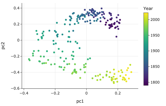
We see a clear difference in speeches over time—speeches given in the 1800s used very different words than speeches given after 2000. It’s also interesting to see that the speeches cluster tightly in the same time period. This suggests that speeches within the same period sound relatively similar, even though the speakers were from different political parties.
This section gave a whirlwind introduction to text analysis. We used text manipulation tools from previous sections to clean up the presidential speeches. Then we used more advanced techniques like stemming, the tf-idf transform, and principal component analysis to compare speeches. Although we don’t have enough space in this book to cover all of these techniques in detail, we hope that this section piqued your interest in the exciting world of text analysis.