Variants of Gradient Descent
Contents
20.4. Variants of Gradient Descent#
Two variants of gradient descent, stochastic gradient descent and mini-batch gradient descent, use subsets of the data when computing the gradient of the average loss and are useful for optimization problems with large datasets. A third alternative, Newton’s method, assumes the loss function is twice differentiable and uses a quadratic approximation to the loss function, rather than the linear approximation used in gradient descent.
Recall that gradient descent takes steps based on the gradient. At step \( t \), we move from \( \boldsymbol{\theta}^{(t)} \) to:
And since \(\nabla_{\theta} L(\boldsymbol{\theta}, \textbf{X}, \textbf{y})\) can be expressed as the average gradient of the loss function \(\cal l\), we have:
This representation of the gradient of the average loss in terms of the average of the gradient of loss at each point in the data shows why the algorithm is also called batch gradient descent. Two variants to batch gradient descent use smaller amounts of the data rather than the complete “batch.” The first, stochastic gradient descent, uses only one observation in each step of the algorithm.
20.4.1. Stochastic Gradient Descent#
Although batch gradient descent can often find an optimal \( \boldsymbol{\theta} \) in relatively few iterations, each iteration can take a long time to compute if the dataset contains many observations. To get around this difficulty, stochastic gradient descent approximates the overall gradient by a single, randomly chosen data point. Since this observation is chosen randomly, we expect that using the gradient at randomly chosen observations will, on average, move in the correct direction and so eventually converge to the minimizing parameter.
In short, to conduct stochastic gradient descent, we replace the average gradient with the gradient at a single data point. So, the update formula is just:
In this formula, the \( i^{th} \) observations \( (\textbf{x}_i, y_i) \) are chosen randomly from the data. Choosing the points randomly is critical to the success of stochastic gradient descent. If the points are not chosen randomly, the algorithm may produce significantly worse results than batch gradient descent.
We most commonly run stochastic gradient descent by randomly shuffling all of the data points and using each point in its shuffled order until we complete one entire pass through the data. If the algorithm hasn’t converged yet, then we reshuffle the points and run another pass through the data. Each iteration of stochastic gradient descent looks at one data point; each complete pass through the data is called an epoch.
Since stochastic descent only examines a single data point at a time, at times it takes steps away from the minimizer, \( \hat{\boldsymbol{\theta}} \), but on average these steps are in the right direction. And since the algorithm computes an update much more quickly than batch gradient descent, it can make significant progress toward the optimal \( \boldsymbol{\hat{\theta}} \) by the time batch gradient descent finishes a single update.
20.4.2. Mini-Batch Gradient Descent#
As its name suggests, mini-batch gradient descent strikes a balance between batch gradient descent and stochastic gradient descent by increasing the number of observations selected at random at each iteration. In mini-batch gradient descent, we average the gradient of the loss function at a few data points instead of at a single point or all the points. We let \(\mathcal{B}\) represent the mini-batch of data points that are randomly sampled from the dataset, and we define the algorithm’s next step as:
As with stochastic gradient descent, we perform mini-batch gradient descent by randomly shuffling the data. Then we split the data into consecutive mini-batches and iterate through the batches in sequence. After each epoch, we reshuffle our data and select new mini-batches.
While we have made the distinction between stochastic and mini-batch gradient descent, stochastic gradient descent is sometimes used as an umbrella term that encompasses the selection of a mini-batch of any size.
Another common optimization technique is Newton’s method.
20.4.3. Newton’s Method#
Newton’s method uses the second derivative to optimize the loss. The basic idea is to approximate the average loss, \( L( \boldsymbol{\theta}) \), in small neighborhoods of \( \boldsymbol{\theta} \), with a quadratic curve rather than a linear approximation. The approximation looks as follows for a small step \( \mathbf{s} \):
where \( g(\boldsymbol{\theta}) = \nabla_{\theta} L(\boldsymbol{\theta}) \) is the gradient and \( H(\boldsymbol{\theta}) = \nabla_{\theta}^2 L(\boldsymbol{\theta}) \) is the Hessian of \( L(\boldsymbol{\theta}) \). More specifically, \( H \) is a \( p \times p \) matrix of second-order partial derivatives in \( \boldsymbol{\theta} \) with \( i \), \( j \) elements:
This quadratic approximation to \( L(\boldsymbol{\theta} + \mathbf{s}) \) has a minimum at \( \mathbf{s} = - [H^{-1} (\boldsymbol{\theta})]g(\boldsymbol{\theta}) \). (Convexity implies that \( H \) is a symmetric square matrix that can be inverted.) Then a step in the algorithm moves from \( \boldsymbol{\theta}^{(t)} \) to:
Figure 20.5 gives the idea behind Newton’s method of optimization.
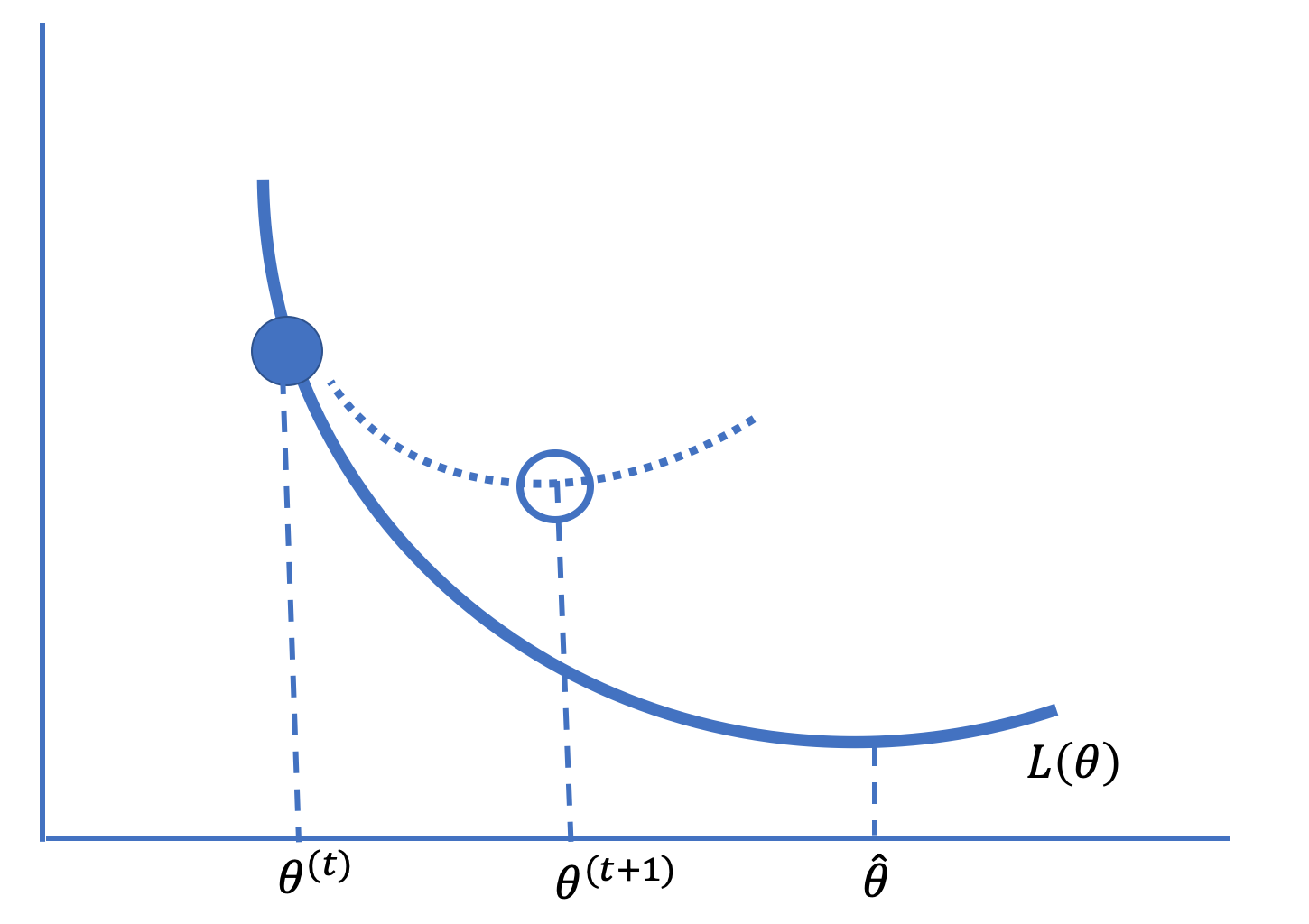
Fig. 20.5 Newton’s method uses a local quadratic approximation to the curve to take steps toward the minimizing value of a convex, twice-differentiable function#
This technique converges quickly if the approximation is accurate and the steps are small. Otherwise, Newton’s method can diverge, which often happens if the function is nearly flat in a dimension. When the function is relatively flat, the derivative is near zero and its inverse can be quite large. Large steps can move to \( \boldsymbol{\theta} \) that are far from where the approximation is accurate. (Unlike with gradient descent, there is no learning rate that keeps steps small.)