20.1. Gradient Descent Basics

Gradient descent is based on the notion that for many loss functions, the function is roughly linear in small neighborhoods of the parameter. Figure 20.2 gives a diagram of the basic idea.

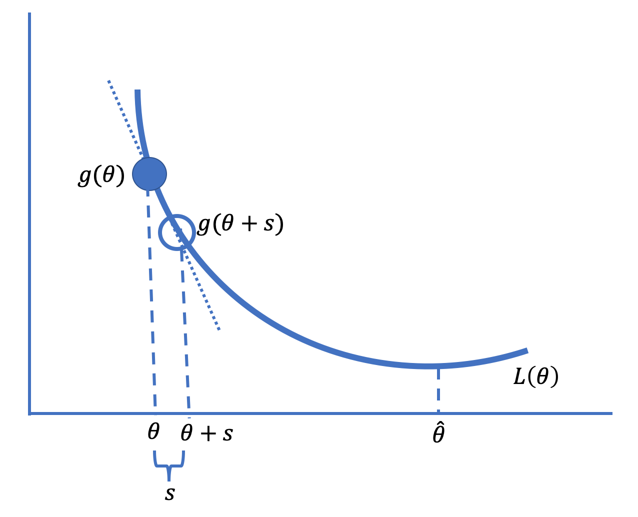
Fig. 20.2 The technique of gradient descent moves in small increments toward the minimizing parameter value

In the diagram, we have drawn the tangent line to the loss curve \( L \) at some point \( {\theta} \) to the left of the minimizing value, \( \hat{\theta} \). Notice that the slope of the tangent line is negative. A short step to the right of \( {\theta} \) to \( {\theta}+\textrm{s} \), for some small amount \( \textrm{s} \), gives a point on the tangent line close to the loss at \( {\theta}+\textrm{s} \), and this loss is smaller than \( L(\tilde{\theta}) \). That is, since the slope, \( b \), is negative, and the tangent line approximates the loss function in a neighborhood of \( {\theta} \), we have:

\[ L({\theta} + \textrm{s}) \approx L(\theta) + b\times\textrm{s} < L(\theta) \]

So, taking a small step to the right of this \( {\theta} \) decreases the loss. On the other hand, on the other side of \( \hat\theta \) in the diagram in Figure 20.2, the slope is positive, and taking a small step to the left decreases the loss.

When we take repeated small steps in the direction indicated by whether the slope of the tangent line is positive or negative at each new step, this leads to smaller and smaller values of the average loss and eventually brings us to the minimizing value \( \hat{\theta} \) (or very close to it). This is the basic idea behind gradient descent.

More formally, to minimize \( L (\boldsymbol{\theta}) \) for a general vector of parameters, \( \boldsymbol{\theta} \), the gradient (first-order partial derivative) determines the direction and size of the step to take. If we write the gradient, \( \nabla_\theta L(\boldsymbol{\theta}) \), as simply \( g( \boldsymbol{\theta})\), then gradient descent says the increment or step is \( -\alpha g( \boldsymbol{\theta}) \) for some small positive \( \alpha \). Then the average loss at the new position is:

\[\begin{split} \begin{aligned} L(\theta + (-\alpha g( \boldsymbol{\theta})) & \approx L(\theta) - \alpha g( \boldsymbol{\theta})^T g( \boldsymbol{\theta}) \\ & < L(\theta) \end{aligned} \end{split}\]

Note that \( g( \boldsymbol{\theta})\) is a \(p \times 1 \) vector and \( g( \boldsymbol{\theta})^T g( \boldsymbol{\theta}) \) is positive.

The steps in the gradient descent algorithm go as follows:

1. Choose a starting value, called \( \boldsymbol{\theta}^{(0)} \) (a common choice is \( \boldsymbol{\theta}^{(0)} = 0 \)).

2. Compute \( \boldsymbol{\theta}^{(t+1)} = \boldsymbol{\theta}^{(t)} - \alpha g( \boldsymbol{\theta}) \).

3. Repeat step 2 until \( \boldsymbol{\theta}^{(t+1)} \) doesn’t change (or changes little) between iterations.

The quantity \( \alpha \) is called the learning rate. Setting \( \alpha \) can be tricky. It needs to be small enough to not overshoot the minimum but large enough to arrive at the minimum in reasonably few steps (see {numref}Figure %s <gd-learning-rate>). There are many strategies for setting \( \alpha \). For example, it can be useful to decrease \( \alpha \) over time. When \( \alpha \) changes between iterations, we use the notation \( \alpha^{(t)} \) to indicate that the learning rate varies during the search.

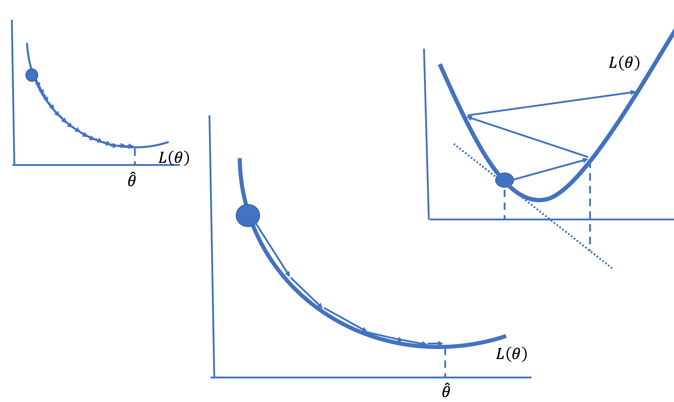
Fig. 20.3 A small learning rate requires many steps to converge (left), and a large learning rate can diverge (right); choosing the learning rate well leads to fast convergence on the minimizing value (middle)

The gradient descent algorithm is simple yet powerful since we can use it for many types of models and many types of loss functions. It is the computational tool of choice for fitting many models, including linear regression on large datasets and logistic regression. We demonstrate the algorithm to fit a constant to the bus delay data (from Chapter 4) next.