Convex and Differentiable Loss Functions
20.3. Convex and Differentiable Loss Functions#
As its name suggests, the gradient descent algorithm requires the function being minimized to be differentiable. The gradient, \( \nabla_\theta L( \boldsymbol{\theta} ) \), allows us to make a linear approximation to the average loss in small neighborhoods of \( \boldsymbol{\theta} \). This approximation gives us the direction (and size) of the step, and as long as we don’t overshoot the minimum, \( \boldsymbol{\hat{\theta}} \), we are bound to eventually reach it. Well, as long as the loss function is also convex.
The step-by-step search for the minimum also relies on the loss function being convex. The function in the diagram on the left in Figure 20.4 is convex, but the function on the right is not. The function on the right has a local minimum, and depending on where the algorithm starts, it might converge to this local minimum and miss the real minimum entirely. The property of convexity avoids this problem. A convex function avoids the problem of local minima. So, with an appropriate step size, gradient descent finds the globally optimal \( \theta \) for any convex, differentiable function.
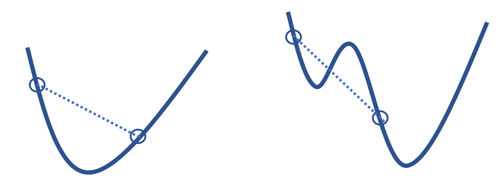
Fig. 20.4 With nonconvex functions (right), gradient descent might locate a local minimum rather than a global minimum, which is not possible with convex functions (left)#
Formally, a function \( f \) is convex if for any two input values, \( \boldsymbol{\theta}_a \) and \( \boldsymbol{\theta}_b \), and any \( q \) between 0 and 1:
This inequality implies that any line segment that connects two points of the function must reside on or above the function itself. Heuristically, this means that whenever we take a small enough step to the right when the gradient is negative or to the left when the gradient is positive, we will head in the direction of the function’s minimum.
The formal definition of convexity gives us a precise way to determine whether a function is convex. And we can use this definition to connect the convexity of the average loss \( L( \boldsymbol{\theta} ) \) to the loss function \( \cal{l}( \boldsymbol{\theta} ) \). We have so far in this chapter simplified the representation of \( L( \boldsymbol{\theta} ) \) by not mentioning the data. Recall:
where \( \textbf{X} \) is an \( n \times p \) design matrix and \( \mathbf{x}_i \) is the \(i\)th row of the design matrix, which corresponds to the \( i \)th observation in the dataset. This means that the gradient can be expressed as follows:
If \( \cal{l}(\boldsymbol{\theta}, \mathbf{x}_i, y_i) \) is a convex function of \( \boldsymbol{\theta} \), then the average loss is also convex. And similarly for the derivative: the derivative of \( \cal{l}(\boldsymbol{\theta}, \mathbf{x}_i, y_i) \) is averaged over the data to evaluate the derivative of \( L(\boldsymbol{\theta}, \textbf{X}, \mathbf{y}) \). We walk through a proof of the convexity property in the exercises.
Now, with a large amount of data, calculating \( \theta^{(t)}\) can be computationally expensive since it involves the average of the gradient \( \nabla_{\theta} {\cal l} \) over all the \( (\textbf{x}_i, y_i) \). We next consider variants of gradient descent that can be computationally faster because they don’t average over all of the data.