Table Shape and Granularity
Contents
8.6. Table Shape and Granularity#
As described earlier, we refer to a dataset’s structure as a mental representation of the data, and in particular, we represent data that have a table structure by arranging values in rows and columns. We use the term granularity to describe what each row in the table represents, and the term shape quantifies the table’s rows and columns.
Now that we have determined the format of the restaurant-related files, we load them into dataframes and examine their shapes:
bus = pd.read_csv('data/businesses.csv', encoding='ISO-8859-1')
insp = pd.read_csv("data/inspections.csv")
viol = pd.read_csv("data/violations.csv")
print(" Businesses:", bus.shape, "\t Inspections:", insp.shape,
     "\t Violations:", viol.shape)
Businesses: (6406, 9) Inspections: (14222, 4) Violations: (39042, 3)
We find that the table with the restaurant information (the business table) has 6,406 rows and 9 columns. Now let’s figure out the granularity of this table. To start, we can look at the first two rows:
| business_id | name | address | city | ... | postal_code | latitude | longitude | phone_number | |
|---|---|---|---|---|---|---|---|---|---|
| 0 | 19 | NRGIZE LIFESTYLE CAFE | 1200 VAN NESS AVE, 3RD FLOOR | San Francisco | ... | 94109 | 37.79 | -122.42 | +14157763262 |
| 1 | 24 | OMNI S.F. HOTEL - 2ND FLOOR PANTRY | 500 CALIFORNIA ST, 2ND FLOOR | San Francisco | ... | 94104 | 37.79 | -122.40 | +14156779494 |
2 rows × 9 columns
These two rows give us the impression that each record represents a particular restaurant. But, we can’t tell from just two records whether or not this is the case. The field named business_id implies that it is the unique identifier for the restaurant. We can confirm this by checking whether the number of records in the dataframe matches the number of unique values in the field business_id:
print("Number of records:", len(bus))
print("Number of unique business ids:", len(bus['business_id'].unique()))
Number of records: 6406
Number of unique business ids: 6406
The number of unique business_ids matches the number of rows in the table, so it seems safe to assume that each row represents a restaurant. Since business_id uniquely identifies each record in the dataframe, we treat business_id as the primary key for the table. We can use primary keys to join tables (see Chapter 6).
Sometimes a primary key consists of two (or more) features.
This is the case for the other two restaurant files.
Let’s continue the examination of the inspections and violations dataframes
and find their granularity.
8.6.1. Granularity of Restaurant Inspections and Violations#
We just saw that there are many more rows in the inspection table compared to the business table. Let’s take a closer look at the first few inspections:
| business_id | score | date | type | |
|---|---|---|---|---|
| 0 | 19 | 94 | 20160513 | routine |
| 1 | 19 | 94 | 20171211 | routine |
| 2 | 24 | 98 | 20171101 | routine |
| 3 | 24 | 98 | 20161005 | routine |
(insp
 .groupby(['business_id', 'date'])
 .size()
 .sort_values(ascending=False)
 .head(5)
)
business_id  date
64859        20150924    2
87440        20160801    2
77427        20170706    2
19           20160513    1
71416        20171213    1
dtype: int64
The combination of restaurant ID and inspection date uniquely identifies each record in this table, with the exception of three restaurants that have two records for their ID-date combination. Let’s examine the rows for restaurant 64859:
insp.query('business_id == 64859 and date == 20150924')
| business_id | score | date | type | |
|---|---|---|---|---|
| 7742 | 64859 | 96 | 20150924 | routine |
| 7744 | 64859 | 91 | 20150924 | routine |
This restaurant got two different inspection scores on the same day! How could this happen? It may be that the restaurant had two inspections in one day, or it might be an error. We address these sorts of questions when we consider the data quality in Chapter 9. Since there are only three of these double-inspection days, we can ignore the issue until we clean the data. So the primary key would be the combination of restaurant ID and inspection date if same-day inspections are removed from the table.
Note that the business_id field in the inspections table acts as a reference to the primary key in the business table.
So business_id in insp is a foreign key because it
links each record in the inspections table to a record in the business table.
This means that we can readily join these two tables together.
Next, we examine the granularity of the third table, the one that contains the violations:
| business_id | date | description | |
|---|---|---|---|
| 0 | 19 | 20171211 | Inadequate food safety knowledge or lack of ce... |
| 1 | 19 | 20171211 | Unapproved or unmaintained equipment or utensils |
| 2 | 19 | 20160513 | Unapproved or unmaintained equipment or utensi... |
| ... | ... | ... | ... |
| 39039 | 94231 | 20171214 | High risk vermin infestation [ date violation... |
| 39040 | 94231 | 20171214 | Moderate risk food holding temperature [ dat... |
| 39041 | 94231 | 20171214 | Wiping cloths not clean or properly stored or ... |
39042 rows × 3 columns
Looking at the first few records in this table, we see that each inspection has multiple entries. The granularity appears to be at the level of a violation found in an inspection. Reading the descriptions, we see that if corrected, a date is listed in the description within square brackets:
viol.loc[39039, 'description']
'High risk vermin infestation [ date violation corrected: 12/15/2017 ]'
In brief, we have found that the three food safety tables have different granularities. Since we have identified primary and foreign keys for them, we can potentially join these tables. If we are interested in studying inspections, we can join the violations and inspections together using the business ID and inspection date. This would let us connect the number of violations found during an inspection to the inspection score.
We can also reduce the inspection table to one per restaurant by selecting the most recent inspection for each restaurant. This reduced data table essentially has a granularity of restaurant and may be useful for a restaurant-based analysis. In Chapter 9, we cover these kinds of actions that reshape a data table, transform columns, and create new columns.
We conclude this section with a look at the shape and granularity of the DAWN survey data.
8.6.2. DAWN Survey Shape and Granularity#
As noted earlier in this chapter, the DAWN file has fixed-width formatting, and we need to rely on a codebook to find out where the fields are. As an example, a snippet of the codebook in Figure 8.2 tells us that age appears in positions 34 and 35 in a row, and it is categorized into 11 age groups: 1 stands for age 5 and under, 2 for ages 6 to 11, …, and 11 for ages 65 and older. Also,–8 represents a missing value.
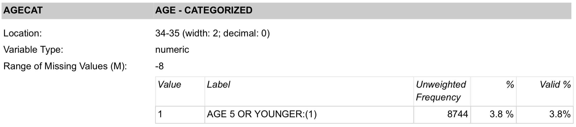
Fig. 8.2 Screenshot of a portion of the DAWN coding for age#
Earlier, we determined that the file contains 200,000 lines and over 280 million characters, so on average, there are about 1,200 characters per line. This might be why they used a fixed-width rather than a CSV format. Think how much larger the file would be if there was a comma between every field!
Given the tremendous amount of information on each line, let’s read just a few
features into a dataframe. We can use the pandas.read_fwf method to do this. We specify the exact positions of the fields to extract, and we provide names for these fields and other information about the header and index:
colspecs = [(0,6), (14,29), (33,35), (35, 37), (37, 39), (1213, 1214)]
varNames = ["id", "wt", "age", "sex", "race","type"]
dawn = pd.read_fwf('data/DAWN-Data.txt', colspecs=colspecs,
                   header=None, index_col=0, names=varNames)
| wt | age | sex | race | type | |
|---|---|---|---|---|---|
| id | |||||
| 1 | 0.94 | 4 | 1 | 2 | 8 |
| 2 | 5.99 | 11 | 1 | 3 | 4 |
| 3 | 4.72 | 11 | 2 | 2 | 4 |
| 4 | 4.08 | 2 | 1 | 3 | 4 |
| 5 | 5.18 | 6 | 1 | 3 | 8 |
We can compare the rows in the table to the number of lines in the file:
dawn.shape
(229211, 5)
The number of rows in the dataframe matches the number of lines in the file. That’s good.
The granularity of the dataframe is a bit complicated due to the survey design. Recall that these data are part of a large scientific study, with a complex sampling scheme. A row represents an emergency room visit, so the granularity is at the emergency room visit level. However, in order to reflect the sampling scheme and be representative of the population of all drug-related ER visits in a year, weights are provided. We must apply the weight to each record when we compute summary statistics, build histograms, and fit models. (The wt field contains these values.)
The weights take into account the chance of an ER visit like this one appearing in the sample. By “like this one” we mean a visit with similar features, such as the visitor age, race, visit location, and time of day. Let’s examine the different values in wt:
dawn['wt'].value_counts()
wt
0.94     1719
84.26    1617
1.72     1435
         ...
1.51        1
3.31        1
3.33        1
Name: count, Length: 3500, dtype: int64
Note
What do these weights mean? As a simplified example, suppose you ran a survey and 45% of your respondents were under 18 years of age, but according to the US Census Bureau, only 22% of the population is under 18. You can adjust your survey responses to reflect the US population by using a small weight (22/45) for those under 18 and a larger weight (78/55) for those 18 and older. To see how we might use these weights, suppose the respondents are asked whether they use Facebook:
< 18 |
18+ |
Total |
|
|---|---|---|---|
No |
1 |
19 |
21 |
Yes |
44 |
35 |
79 |
Total |
45 |
55 |
100 |
Overall, 79% of the respondents say they are Facebook users, but the sample is skewed toward the younger generation. We can adjust the estimate with the weights so that the age groups match the population. Then the adjusted percentage of Facebook users drops to:
The DAWN survey uses the same idea, except that it splits the groups much more finely.
It is critical to include the survey weights in your analysis to get data that represents the population at large. For example, we can compare the calculation of the proportion of females among the ER visits both with and without the weights:
print(f'Unweighted percent female: {np.average(dawn["sex"] == 2):.1%}')
print(f'  Weighted percent female:',
      f'{np.average(dawn["sex"] == 2, weights=dawn["wt"]):.1%}')
Unweighted percent female: 48.0%
  Weighted percent female: 52.3%
These figures differ by more than 4 percentage points. The weighted version is a more accurate estimate of the proportion of females among the entire population of drug-related ER visits.
Sometimes the granularity can be tricky to figure out, like we saw with the inspections data. And at other times, we need to take sampling weights into account, like for the DAWN data. These examples show it’s important to take your time and review the data descriptions before proceeding with analysis.