17.3. Bootstrapping for Inference

In many hypothesis tests the assumptions of the null hypothesis lead to a complete specification of a hypothetical population and data design (see Figure 17.1), and we use this specification to simulate the sampling distribution of a statistic. For example, the rank test for the Wikipedia experiment led us to sampling the integers 1, …, 200, which we easily simulated. Unfortunately, we can’t always specify the population and model completely. To remedy the situation, we substitute the data for the population. This substitution is at the heart of the notion of the bootstrap. Figure 17.2 updates Figure 17.1 to reflect this idea; here the population distribution is replaced by the empirical distribution to create what is called the bootstrap population.

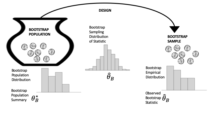
Fig. 17.2 Diagram of bootstrapping the data generation process

The rationale for the bootstrap goes like this:

• Your sample looks like the population because it is a representative sample, so we replace the population with the sample and call it the bootstrap population.

• Use the same data generation process that produced the original sample to get a new sample, which is called a bootstrap sample, to reflect the change in the population. Calculate the statistic on the bootstrap sample in the same manner as before and call it the bootstrap statistic. The bootstrap sampling distribution of the bootstrap statistic should be similar in shape and spread to the true sampling distribution of the statistic.

• Simulate the data generation process many times, using the bootstrap population, to get bootstrap samples and their bootstrap statistics. The distribution of the simulated bootstrap statistics approximates the bootstrap sampling distribution of the bootstrap statistic, which itself approximates the original sampling distribution.

Take a close look at Figure 17.2 and compare it to Figure 17.1. Essentially, the bootstrap simulation involves two approximations: the original sample approximates the population, and the simulation approximates the sampling distribution. We have been using the second approximation in our examples so far; the approximation of the population by the sample is the core notion behind bootstrapping. Notice that in Figure 17-2, the distribution of the bootstrap population (on the left) looks like the original sample histogram; the sampling distribution (in the middle) is still a probability distribution based on the same data generation process as in the original study, but it now uses the bootstrap population; and the sample distribution (on the right) is a histogram of one sample taken from the bootstrap population.

You might be wondering how to take a simple random sample from your bootstrap population and not wind up with the exact same sample each time. After all, if your sample has 100 units in it and you use it as your bootstrap population, then 100 draws from the bootstrap population without replacement will take all of the units and give you the same bootstrap sample every time. There are two approaches to solving this problem:

1. When sampling from the bootstrap population, draw units from the bootstrap population with replacement. Essentially, if the original population is very large, then there is little difference between sampling with and without replacement. This is the more common approach by far.

2. “Blow up the sample” to be the same size as the original population. That is, tally the fraction of each unique value in the sample, and add units to the bootstrap population so that it is the same size as the original population, while maintaining the proportions. For example, if the sample is size 30 and 1/3 of the sample values are 0, then a bootstrap population of 750 should include 250 zeros. Once you have this bootstrap population, use the original data generation procedure to take the bootstrap samples.

The example of vaccine efficacy used a bootstrap-like process, called the parameterized bootstrap. Our null model specified 0-1 urns, but we didn’t know how many 0s and 1s to put in the urn. We used the sample to determine the proportions of 0s and 1s; that is, the sample specified the parameters of the multivariate hypergeometric. Next, we use the example of calibrating air quality monitors to show how bootstrapping could be used to test a hypothesis.

Warning

It’s a common mistake to think that the center of the bootstrap sampling distribution is the same as the center of the true sampling distribution. If the mean of the sample is not 0, then the mean of the bootstrap population is also not 0. That’s why we use the spread of the bootstrap distribution, and not its center, in hypothesis testing. The next example shows how we might use the bootstrap to test a hypothesis.

The case study on calibrating air quality monitors (see Chapter 12) fit a model to adjust the measurements from an inexpensive monitor to more accurately reflect true air quality. This adjustment included a term in the model related to humidity. The fitted coefficient was about \(0.2\) so that on days of high humidity the measurement is adjusted upward more than on days of low humidity. However, this coefficient is close to 0, and we might wonder whether including humidity in the model is really needed. In other words, we want to test the hypothesis that the coefficient for humidity in the linear model is 0. Unfortunately, we can’t fully specify the model, because it is based on measurements taken over a particular time period from a set of air monitors (both PurpleAir and those maintained by the EPA). This is where the bootstrap can help.

Our model makes the assumption that the air quality measurements taken resemble the population of measurements. Note that weather conditions, the time of year, and the location of the monitors make this statement a bit hand-wavy; what we mean here is that the measurements are similar to others taken under the same conditions as those when the original measurements were taken. Also, since we can imagine a virtually infinite supply of air quality measurements, we think of the procedure for generating measurements as draws with replacement from the urn. Recall that in Chapter 2 we modeled the urn as repeated draws with replacement from an urn of measurement errors. This situation is a bit different because we are also including the other factors mentioned already (weather, season, location).

Our model is focused on the coefficient for humidity in the linear model:

\[ \begin{aligned} \text{PA} \approx \theta_0 + \theta_1 \text{AQ} + \theta_2 \text{RH} \end{aligned} \]

Here, \(\text{PA}\) refers to the PurpleAir PM2.5 measurement, \( \text{RH}\) is the relative humidity, and \(\text{AQ}\) stands for the more exact measurement of PM2.5 made by the more accurate AQS monitors. The null hypothesis is \(\theta_2 = 0\); that is, the null model is the simpler model:

\[ \begin{aligned} \text{PA} \approx \theta_0 + \theta_1 \text{AQ} \end{aligned} \]

To estimate \(\theta_2\), we use the linear model fitting procedure from Chapter 15.

Our bootstrap population consists of the measurements from Georgia that we used in Chapter 15. Now we sample rows from the data frame (which is equivalent to our urn) with replacement using the chance mechanism randint. This function takes random samples with replacement from a set of integers. We use the random sample of indices to create the bootstrap sample from the data frame. Then we fit the linear model and get the coefficient for humidity (our bootstrap statistic). The following boot_stat function performs this simulation process:

from scipy.stats import randint

def boot_stat(X, y):
    n = len(X)
    bootstrap_indexes = randint.rvs(low=0, high=(n - 1), size=n)
    theta2 = (
        LinearRegression()
        .fit(X.iloc[bootstrap_indexes, :], y.iloc[bootstrap_indexes])
        .coef_[1]
    )
    return theta2

We set up the design matrix and the outcome variable and check our boot_stat function once to test it:

X = GA[['pm25aqs', 'rh']]
y = GA['pm25pa']

boot_stat(X, y)

0.21572251745549495

When we repeat this process 10,000 times, we get an approximation to the bootstrap sampling distribution of the bootstrap statistic (the fitted humidity coefficient):

np.random.seed(42)
boot_theta_hat = np.array([boot_stat(X, y) for _ in range(10_000)])

We are interested in the shape and spread of this bootstrap sampling distribution (we know that the center will be close to the original coefficient of \(0.21\)):

px.histogram(x=boot_theta_hat, nbins=50,
             labels=dict(x='Bootstrapped humidity coefficient'),
             width=350, height=250)

By design, the center of the bootstrap sampling distribution will be near \(\hat{\theta}\) because the bootstrap population consists of the observed data. So, rather than compute the chance of a value at least as large as the observed statistic, we find the chance of a value at least as small as 0. The hypothesized value of 0 is far from the sampling distribution.

None of the 10,000 simulated regression coefficients are as small as the hypothesized coefficient. Statistical logic leads us to reject the null hypothesis that we do not need to adjust the model for humidity.

The form of the hypothesis test we performed here looks different than the earlier tests because the sampling distribution of the statistic is not centered on the null. That is because we are using the bootstrap to create the sampling distribution. We are, in effect, using a confidence interval for the coefficient to test the hypothesis. In the next section we introduce interval estimates more generally, including those based on the bootstrap, and we connect the concepts of hypothesis testing and confidence intervals.