Numerical Optimization
20. Numerical Optimization#
At this point in the book, our modeling procedure should feel familiar: we define a model, choose a loss function, and fit the model by minimizing the average loss over our training data. We’ve seen several techniques to minimize loss. For example, we used both calculus and a geometric argument in Chapter 15 to find a simple expression for fitting linear models using squared loss.
But empirical loss minimization isn’t always so straightforward. Lasso regression, with the addition of the \( L_1 \) penalty to the average squared loss, no longer has a closed form solution, and logistic regression uses cross-entropy loss to fit a nonlinear model. In these cases, we use numerical optimization to fit the model, where we systematically choose parameter values to evaluate the average loss in search of the minimizing value.
When we introduced loss functions in Chapter 4, we performed a simple numerical optimization to find the minimizer of the average loss. We created a grid of \( \theta \) values and evaluated the average loss at all points in the grid (see Figure 20.1 for a diagram of this concept). The grid point with the smallest average loss we took as the best fit. Unfortunately, this sort of grid search quickly becomes impractical, for the following reasons:
For complex models with many features, the grid becomes unwieldy. With only four features and a grid of 100 values for each feature, we must evaluate the average loss at \( 100^4 = 100,000,000 \) grid points.
The range of parameter values to search over must be specified in advance to create the grid, and when we don’t have a good sense of the range, we need to start with a wide grid and possibly repeat the grid search over narrower ranges.
With a large number of observations, the evaluation of the average loss over the grid points can be slow.
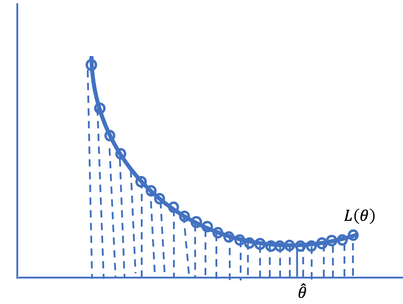
Fig. 20.1 Searching over a grid of points can be computationally slow or inexact#
In this chapter, we introduce numerical optimization techniques that take advantage of the shape and smoothness of the loss function in the search for the minimizing parameter values. We first introduce the basic idea behind the technique of gradient descent, then we give an example and describe the properties of the loss function that make gradient descent work, and finally, we provide a few extensions of gradient descent.