Probability Review
Contents
Probability Review#
Many fundamental aspects of data science, including data design, rely on uncertain phenomenon. The laws of probability allow us to quantify this uncertainty. In this section, we will provide a quick review of important probability concepts for this course.
Suppose we toss two coins with one side labeled heads (\(H\)) and the other labeled tails (\(T\)). We call the action of tossing the coins and observing the results our experiment. The outcome space \(\Omega\) consists of all the possible outcomes of an experiment. In this experiment, our outcome space consists of the following outcomes: \(\Omega = \{HH, HT, TH, TT\}\).
An event is any subset of the outcome space. For example, “getting one tails and one heads” is an event for the coin toss experiment. This event consists of the outcomes \(\{HT, TH\}\). We use the notation \(P(\text{event})\) to represent the probability of an event occurring, in this case, \(P(\text{one heads and one tails})\).
Probability of Events#
In this course, we will typically deal with outcome spaces where each outcome is equally likely to occur. These spaces have simple probability calculations. The probability of an event occurring is equal to the proportion of outcomes in the event, or the number of outcomes in the event divided by the total number of outcomes in the outcome space:
In the coin toss experiment, the events \(\{HH, HT, TH, TT\}\) are all equally likely to occur. To calculate \(P(\text{one heads and one tails})\), we see that there are two outcomes in the event and four outcomes total:
There are three fundamental axioms of probability:
The probability of an event is a real number between 0 and 1, inclusive: \(0 \leq P(\text{event}) \leq 1\).
The probability of the entire outcome space is 1: \(P(\Omega) = 1\).
The third axiom involves mutually exclusive events.
A or B#
We often want to calculate the probability that event \(A\) or event \(B\) occurs. For example, a polling agency might want to know the probability that a randomly selected US citizen is either 17 or 18 years old.
We state that events are mutually exclusive when at most one of them can happen. If \(A\) is the event that we select an 17-year-old and \(B\) is the event that we select a 18-year old, \(A\) and \(B\) are mutually exclusive because a person cannot be both 17 and 18 at the same time.
The probability \(P(A \cup B)\) that \(A\) or \(B\) occurs is simple to calculate when \(A\) and \(B\) are mutually exclusive:
This is the third axiom of probability, the addition rule.
In the 2010 census, 1.4% of US citizens were 17 years old and 1.5% were 18. Thus, for a randomly chosen US citizen in 2010, \(P(A) = 0.014\) and \(P(B) = 0.015\), giving \( P(A \cup B) = P(A) + P(B) = 0.029 \).
To understand this rule, consider the following Venn diagram from the Prob 140 textbook:
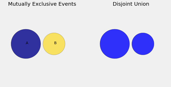
When events \(A\) and \(B\) are mutually exclusive, there are no outcomes that appear in both \(A\) and \(B\). Thus, if \(A\) has 5 possible outcomes and \(B\) has 4 possible outcomes, we know that the event \(A \cup B\) has 9 possible outcomes.
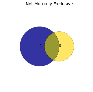
Unfortunately, when \(A\) and \(B\) are not mutually exclusive, the simple addition rule does not apply. Suppose we want to calculate the probability that in two coin flips, exactly one flip is heads or exactly one flip is tails.
If \(A\) is the event that exactly one heads appears, \(P(A) = \frac{2}{4}\) since \(A\) consists of the outcomes \(\{ HT, TH \}\) and there are four outcomes total. If \(B\) is the event that exactly one tails appears, \(P(B) = \frac{2}{4}\) since \(B\) consists of the outcomes \(\{ HT, TH \}\). However, the event \(A \cup B\) only contains two outcomes since the outcomes are the same in both \(A\) and \(B\): \(P(A \cup B) = \frac{1}{2} \). Blindly applying the addition rule results in an incorrect conclusion. There are outcomes that appear in both \(A\) and \(B\); adding the number of outcomes in \(A\) and \(B\) counts them twice. In the image below, we illustrate the fact that the overlapping region of the Venn diagram gets shaded twice, once by \(A\) and once by \(B\).
To compensate for this overlap, we need to subtract out the the probability \(P(A \cap B)\) that both \(A\) and \(B\) occur. To calculate the probability that either of two non-mutually exclusive events occurs, we use:
Notice that when \(A\) and \(B\) are mutually exclusive, \( P(A \cap B) = 0 \) and the equation simplifies to the addition rule above.
A and B#
We also often wish to calculate probability that both event \(A\) and \(B\) occur. Suppose we have a class with only three students, whom we’ll label as \(X\), \(Y\), and \(Z\). What is the probability that drawing a sample of size 2 without replacement results in \(Y\), then \(X\)?
One simple way to calculate this probability is to enumerate the entire outcome space:
Since there our event consists of only one outcome:
We can also calculate this probability by noticing that this event can be broken down into two events that happen in sequence, the event of drawing \(Y\) as the first student, then the event of drawing \(X\) after drawing \(Y\).
The probability of drawing \(Y\) as the first student is \( \frac{1}{3} \) since there are three outcomes in the outcome space (\(X\), \(Y\), and \(Z\)) and our event only contains one.
After drawing \(Y\), the outcome space of the second event only contains \( \{ X, Z \} \). Thus, the probability of drawing \(X\) as the second student is \( \frac{1}{2} \). This probability is called the conditional probability of drawing \(X\) second given that \(Y\) was drawn first. We use the notation \(P(B | A)\) to describe the conditional probability of an event \(B\) occurring given event \(A\) occurs.
Now, observe that:
This happens to be a general rule of probability, the multiplication rule. For any events \(A\) and \(B\), the probability that both \(A\) and \(B\) occur is:
In certain cases, two events may be independent. That is, the probability that \(B\) occurs does not change after \(A\) occurs. For example, the event that a 6 occurs on a dice roll does not affect the probability that a 5 occurs on the next dice roll. If \(A\) and \(B\) are independent, \( P(B | A) = P(B) \). This simplifies our multiplication rule:
Although this simplification is extremely convenient for calculation, many real-world events are not independent even if their relationship is not obvious at a first glance. For example, the event that a randomly selected US citizen is over 90 years old is not independent from the event that the citizen is male—given that the person is over 90, the person is almost twice as likely to be female than male.
As data scientists, we must examine assumptions of independence very closely! The US housing crash of 2008 might have been avoided if the bankers did not assume that housing markets in different cities moved independently of one another (link to an Economist article).