Distributions: Population, Empirical, Sampling
17.1. Distributions: Population, Empirical, Sampling#
The population, sampling, and empirical distributions are important concepts that guide us when we make inferences about a model or predictions for new observations. Figure 17.1 provides a diagram that can help distinguish between them. The diagram uses the notions of population and access frame from Chapter 2 and the urn model from Chapter 3. On the left is the population that we are studying, represented as marbles in an urn with one marble for each unit. We have simplified the situation to where the access frame and the population are the same; that is, we can access every unit in the population. (The problems that arise when this is not the case are covered in Chapters 2 and Chapter 3.) The arrow from the urn to the sample represents the design, meaning the protocol for selecting the sample from the frame. The diagram shows this selection process as a chance mechanism, represented by draws from an urn filled with indistinguishable marbles. On the right side of the diagram, the collection of marbles constitutes our sample (the data we got).
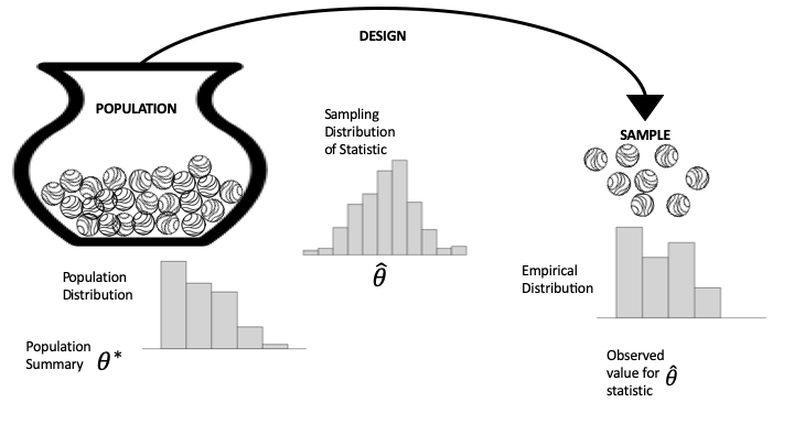
Fig. 17.1 Diagram of the data generation process#
We have kept the diagram simple by considering measurements for just one feature. Below the urn in the diagram is the population histogram for that feature. The population histogram represents the distribution of values across the entire population. On the far right, the empirical histogram shows the distribution of values for our actual sample. Notice that these two distributions are similar in shape. This happens when our sampling mechanism produces representative samples.
We are often interested in a summary of the sample measurements, such as the mean, median, slope from a simple linear model, and so on. Typically, this summary statistic is an estimate for a population parameter, such as the population mean or median. The population parameter is shown as \( \theta^* \) on the left of the diagram; on the right, the summary statistic, calculated from the sample, is \( \hat{\theta} \).
The chance mechanism that generates our sample might well produce a different set of data if we were to conduct our investigation over again. But if the protocols are well designed, we expect the sample to still resemble the population. In other words, we can infer the population parameter from the summary statistic calculated from the sample. The sampling distribution in the middle of the diagram is a probability distribution for the statistic. It shows the possible values that the statistic might take for different samples and their chances. In Chapter 3, we used simulation to estimate the sampling distribution in several examples. In this chapter, we revisit these and other examples from earlier chapters to formalize the analyses.
One last point about these three histograms: as introduced in Chapter 10, the rectangles provide the fraction of observations in any bin. In the case of the population histogram, this is the fraction of the entire population; for the empirical histogram, the area represents the fraction in the sample; and for the sampling distribution, the area represents the chance the data generation mechanism would produce a sample statistic in this bin.
Finally, we typically don’t know the population distribution or parameter, and we try to infer the parameter or predict values for unseen units in the population. At other times, a conjecture about the population can be tested using the sample. Testing is the topic of the next section.