Probability for Inference and Prediction
Contents
17.6. Probability for Inference and Prediction#
Hypothesis testing, confidence intervals, and prediction intervals rely on probability calculations computed from the sampling distribution and the data generation process. These probability frameworks also enable us to run simulation and bootstrap studies for a hypothetical survey, an experiment, or some other chance process in order to study its random behavior. For example, we found the sampling distribution for an average of ranks under the assumption that the treatment in a Wikipedia experiment was not effective. Using simulation, we quantified the typical deviations from the expected outcome and the distribution of the possible values for the summary statistic. The triptych in Figure 1 17.1 provided a diagram to guide us in the process; it helped keep straight the differences between the population, probability, and sample and also showed their connections. In this section, we bring more mathematical rigor to these concepts.
We formally introduce the notions of expected value, standard deviation, and random variable, and we connect them to the concepts we have been using in this chapter for testing hypotheses and making confidence and prediction intervals. We begin with the specific example from the Wikipedia experiment, and then we generalize. Along the way, we connect this formalism to the triptych that we have used as our guide throughout the chapter.
17.6.1. Formalizing the Theory for Average Rank Statistics#
Recall in the Wikipedia experiment that we pooled the post-award productivity values from the treatment and control groups and converted them into ranks, \(1, 2, 3, \ldots, 200\), so the population is simply made up of the integers from 1 to 200. Figure 17.3 is a diagram that represents this specific situation. Notice that the population distribution is flat and ranges from 1 to 200 (left side of Figure 17.3). Also, the population summary (called population parameter) we use is the average rank:
Another relevant summary is the spread about \(\theta^*\), defined as the population standard deviation:
The SD(pop) represents the typical deviation of a rank from the population average. To calculate SD(pop) for this example takes some mathematical handiwork:
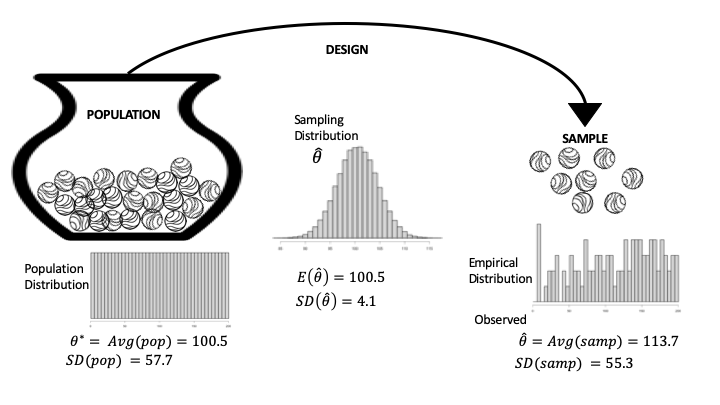
Fig. 17.3 Diagram of the data generation process for the Wikipedia experiment; this is a special case where we know the population#
The observed sample consists of the integer ranks of the treatment group; we refer to these values as \(k_1, k_2, \ldots, k_{100}.\) The sample distribution appears on the right in Figure 17.3 (each of the 100 integers appears once).
The parallel to the population average is the sample average, which is our statistic of interest:
The \(\text{Avg}(\text{sample})\) is the observed value for \(\hat{\theta}\). Similarly, the spread about \(\text{Avg}(\text{sample})\), called the standard deviation of the sample, represents the typical deviation of a rank in the sample from the sample average:
Notice the parallel between the definitions of the sample statistic and the population parameter in the case where they are averages. The parallel between the two SDs is also noteworthy.
Next we turn to the data generation process: draw 100 marbles from the urn (with values \(1, 2,\ldots,200\)), without replacement, to create the treatment ranks. We represent the action of drawing the first marble from the urn, and the integer that we get, by the capital letter \(Z_1\). This \(Z_1\) is called a random variable. It has a probability distribution determined by the urn model. That is, we can list all of the values that \(Z_1\) might take and the probability associated with each:
In this example, the probability distribution of \(Z_1\) is determined by a simple formula because all of the integers are equally likely to be drawn from the urn.
We often summarize the distribution of a random variable by its expected value and standard deviation. Like with the population and sample, these two quantities give us a sense of what to expect as an outcome and how far the actual value might be from what is expected.
For our example, the expected value of \(Z_1\) is simply:
Notice that \(\mathbb{E}[Z_1] = \theta^*\), the population average from the urn. The average value in a population and the expected value of a random variable that represents one draw at random from an urn that contains the population are always the same. This is more easily seen by expressing the population average as an average of the unique values in the population weighted by the fraction of units that have that value. The expected value of a random variable of a draw at random from the population urn uses the exact same weights because they match the chance of selecting the particular value.
Note
The term expected value can be a bit confusing because it need not be a possible value of the random variable. For example, \(\mathbb{E}[Z_1] = 100.5\), but only integers are possible values for \(Z_1\).
Next, the variance of \(Z_1\) is defined as follows:
Additionally:
We again point out that the standard deviation of \(Z_1 \) matches the \(\text{SD}\)(pop).
To describe the entire data generation process in Figure 17.3, we also define \(Z_2 , Z_3, \ldots, Z_{100}\) as the result of the remaining 99 draws from the urn. By symmetry, these random variables should all have the same probability distribution. That is, for any \(k = 1, \ldots, 200\):
This implies that each \(Z_i\) has the same expected value, 100.5, and standard deviation, 57.7. However, these random variables are not independent. For example, if you know that \(Z_1 = 17\), then it is not possible for \(Z_2 = 17\).
To complete the middle portion of Figure 17.3, which involves the sampling distribution of \(\hat{\theta}\), we express the average rank statistic as follows:
We can use the expected value and SD of \(Z_1\) and our knowledge of the data generation process to find the expected value and SD of \(\hat{\theta}\). We first find the expected value of \(\hat{\theta}\):
In other words, the expected value of the average of random draws from the population equals the population average. Here we provide formulas for the variance of the average in terms of the population variance, as well as the SD:
These computations relied on several properties of expected value and variance of a random variable and sums of random variables. Next, we provide properties of sums and averages of random variables that can be used to derive the formulas we just presented.
17.6.2. General Properties of Random Variables#
In general, a random variable represents a numeric outcome of a chance event. In this book, we use capital letters like \(X\) or \(Y\) or \(Z\) to denote a random variable. The probability distribution for \(X\) is the specification \(\mathbb{P}(X = x) = p_x\) for all values \(x\) that the random variable takes on.
Then, the expected value of \(X\) is defined as:
The variance \(X\) is defined as:
And the \(\text{SD}(X)\) is the square root of \(\mathbb{V}(X)\).
Note
Although random variables can represent quantities that are either discrete (such as the number of children in a family drawn at random from a population) or continuous (such as the air quality measured by an air monitor), we address only random variables with discrete outcomes in this book. Since most measurements are made to a certain degree of precision, this simplification doesn’t limit us too much.
Simple formulas provide the expected value, variance, and standard deviation when we make scale and shift changes to random variables, such as \(a + bX\) for constants \(a\) and \(b\):
To convince yourself that these formulas make sense, think about how a distribution changes if you add a constant \(a\) to each value or scale each value by \(b\). Adding \(a\) to each value would simply shift the distribution, which in turn would shift the expected value but not change the size of the deviations about the expected value. On the other hand, scaling the values by, say, 2 would spread the distribution out and essentially double both the expected value and the deviations from the expected value.
We are also interested in the properties of the sum of two or more random variables. Let’s consider two random variables, \(X\) and \(Y\). Then:
But to find the variance of \(a + bX + cY\), we need to know how \(X\) and \(Y\) vary together, which is called the joint distribution of \(X\) and \(Y\). The joint distribution of \(X\) and \(Y\) assigns probabilities to combinations of their outcomes:
A summary of how \(X\) and \(Y\) vary together, called the covariance, is defined as:
The covariance enters into the calculation of \(\mathbf(a + bX + cY)\), as shown here:
In the special case where \(X\) and \(Y\) are independent, their joint distribution is simplified to \(p_{x,y} = p_x p_y\). And in this case, \(Cov(X,Y) = 0\), so:
These properties can be used to show that for random variables \(X_1, X_2, \ldots X_n\) that are independent with expected value \(\mu\) and standard deviation \(\sigma\), the average, \(\bar{X}\), has the following expected value, variance, and standard deviation:
This situation arises with the urn model where \(X_1, \ldots,X_n\) are the result of random draws with replacement. In this case, \(\mu\) represents the average of the urn and \(\sigma\) the standard deviation.
However, when we make random draws from the urn without replacement, the \(X_i\) are not independent. In this situation, \(\bar{X}\) has the following expected value and variance:
Notice that while the expected value is the same as when the draws are without replacement, the variance and SD are smaller. These quantities are adjusted by \((N-n)/(N-1)\), which is called the finite population correction factor. We used this formula earlier to compute the \(SD(\hat{\theta})\) in our Wikipedia example.
Returning to Figure 17.3, we see that the sampling distribution for \(\bar{X}\) in the center of the diagram has an expectation that matches the population average; the SD decreases like \(1/\sqrt{n}\) but even more quickly because we are drawing without replacement; and the distribution is shaped like a normal curve. We saw these properties earlier in our simulation study.
Now that we have outlined the general properties of random variables and their sums, we connect these ideas to testing, confidence, and prediction intervals.
17.6.3. Probability Behind Testing and Intervals#
As mentioned at the beginning of this chapter, probability is the underpinning of conducting a hypothesis test, providing a confidence interval for an estimator and a prediction interval for a future observation.
We now have the technical machinery to explain these concepts, which we have carefully defined in this chapter without the use of formal technicalities. This time we present the results in terms of random variables and their distributions.
Recall that a hypothesis test relies on a null model that provides the probability distribution for the statistic, \(\hat{\theta}\). The tests we carried out were essentially computing (sometimes approximately) the following probability. Given the assumptions of the null distribution:
Oftentimes, the random variable is normalized to make these computations easier and standard:
When \(SD(\hat{\theta})\) is not known, we have approximated it via simulation, and when we have a formula for \(SD(\hat{\theta})\) in terms of \(SD(pop)\), we substitute \(SD(samp)\) for \(SD(pop)\). This normalization is popular because it simplifies the null distribution. For example, if \(\hat{\theta}\) has an approximate normal distribution, then the normalized version will have a standard normal distribution with center 0 and SD 1. These approximations are useful when a lot of hypothesis tests are being carried out, such as with A/B testing, for there is no need to simulate for every statistic because we can just use the normal curve probabilities.
The probability statement behind a confidence interval is quite similar to the probability calculations used in testing. In particular, to create a 95% confidence interval where the sampling distribution of the estimator is roughly normal, we standardize and use the probability:
Note that \(\hat{\theta}\) is a random variable in the preceding probability statement and \(\theta^*\) is considered a fixed unknown parameter value. The confidence interval is created by substituting the observed statistic for \(\hat\theta\) and calling it a 95% confidence interval:
Once the observed statistic is substituted for the random variable, then we say that we are 95% confident that the interval we have created contains the true value \(\theta^*\). In other words, in 100 cases where we compute an interval in this way, we expect 95 of them to cover the population parameter that we are estimating.
Next, we consider prediction intervals. The basic notion is to provide an interval that denotes the expected variation of a future observation about the estimator. In the simple case where the statistic is \(\bar{X}\) and we have a hypothetical new observation \(X_0\) that has the same expected value, say \(\mu\), and standard deviation, say \(\sigma\), of the \(X_i\), then we find the expected variation of the squared loss:
Notice there are two parts to the variation: one due to the variation of \(X_0\) and the other due to the approximation of \(\mathbb{E}(X_0)\) by \(\bar{X}\).
In the case of more complex models, the variation in prediction also breaks down into two components: the inherent variation in the data about the model plus the variation in the sampling distribution due to the estimation of the model. Assuming the model is roughly correct, we can express it as follows:
where \(\boldsymbol{\theta}^*\) is a \((p+1) \times 1\) column vector, \(\textbf{X}\) is an \(n \times (p+1)\) design matrix, and \(\boldsymbol{\epsilon}\) consists of \(n\) independent random variables that each have expected value 0 and variance \(\sigma^2\). In this equation, \(\mathbf{Y}\) is a vector of random variables, where the expected value of each variable is determined by the design matrix and the variance is \(\sigma^2\). That is, the variation about the line is constant in that it does not change with \(\mathbf{x}\).
When we create prediction intervals in regression, they are given a \(1 \times (p+1)\) row vector of covariates, called \(\mathbf{x}_0\). Then the prediction is \(\mathbf{x}_0\boldsymbol{\hat{\theta}}\), where \(\boldsymbol{\hat{\theta}}\) is the estimated parameter vector based on the original \(\mathbf{y}\) and design matrix \(\textbf{X}\). The expected squared error in this prediction is:
We approximate the variance of \(\epsilon\) with the variance of the residuals from the least squares fit.
The prediction intervals we create using the normal curve rely on the additional assumption that the distribution of the errors is approximately normal. This is a stronger assumption than we make for the confidence intervals. With confidence intervals, the probability distribution of \(X_i\) need not look normal for \(\bar{X}\) to have an approximate normal distribution. Similarly, the probability distribution of \(\boldsymbol{\epsilon}\) in the linear model need not look normal for the estimator \(\hat{\theta}\) to have an approximate normal distribution.
We also assume that the linear model is approximately correct when making these prediction intervals. In Chapter 16, we considered the case where the fitted model doesn’t match the model that has produced the data. We now have the technical machinery to derive the model bias–variance trade-off introduced in that chapter. It’s very similar to the prediction interval derivation with a couple of small twists.
17.6.4. Probability Behind Model Selection#
In Chapter 16, we introduced model under- and overfitting with mean square error. We described a general setup where the data might be expressed as follows:
The \(\epsilon\) are assumed to behave like random errors that have no trends or patterns, have constant variance, and are independent of one another. The signal in the model is the function, \(g()\). The data are the \( (\mathbf{x}_i, y_i) \) pairs, and we fit models by minimizing the MSE:
Here \(\cal{F}\) is the collection of models over which we are minimizing. This collection might be all polynomials of degree \(m\) or less, bent lines with a bend at point \(k\), and so on. Note that \(g\) doesn’t have to be in the collection of functions that we are using to fit a model.
Our goal in model selection is to land on a model that predicts a new observation well. For a new observation, we would like the expected loss to be small:
This expectation is with respect to the distribution of possible \((\mathbf{x}_0, y_0)\) and is called risk. Since we don’t know the population distribution of \( (\mathbf{x}_0 , y_0) \), we can’t calculate the risk, but we can approximate it by the average loss over the data we have collected:
This approximation goes by the name of empirical risk. But hopefully you recognize it as mean square error (MSE):
We fit models by minimizing the empirical risk (or MSE) over all possible models, \( \cal{F} = \{ f \} \),
The fitted model is called \( \hat{f} \), a slightly more general representation of the linear model \( \textbf{X}\hat{\boldsymbol{\theta}}\). This technique is aptly called empirical risk minimization.
In Chapter 16, we saw problems arise when we used the empirical risk to both fit a model and evaluate the risk for a new observation. Ideally, we want to estimate the risk (expected loss):
where the expected value is over the new observation \( (\mathbf{x}_0, y_0) \) and over \( {\hat{f}} \) (which involves the original data \( (\textbf{x}_i, {y}_i) \), \( i = 1, \ldots, n \)).
To understand the problem, we decompose this risk into three parts representing the model bias,the model variance, and the irreducible error from \( \epsilon \):
To derive the equality labeled “expanding the square,” we need to formally prove that the cross product terms in the expansion are all 0. This takes a bit of algebra and we don’t present it here. But the main idea is that the terms \(\epsilon_0\) and \((\hat{f}(x_0) - \mathbb{E}[\hat{f}(x_0])\) are independent and both have the expected value 0. The remaining three terms in the final equation—model bias, model variance, and irreducible error—are described as follows:
- Model bias
The first of the three terms in the final equation is model bias (squared). When the signal, \( g \), does not belong to the model space, we have model bias. If the model space can approximate \(g\) well, then the bias is small. Note that this term is not present in our prediction intervals because we assumed that there is no (or minimal) model bias.
- Model variance
The second term represents the variability in the fitted model that comes from the data. We have seen in earlier examples that high-degree polynomials can overfit, and so vary a lot from one set of data to the next. The more complex the model space, the greater the variability in the fitted model.
- Irreducible error
Finally, the last term is the variability in the error, the \(\epsilon_0\), which is dubbed the “irreducible error.” This error sticks around whether we have underfit with a simple model (high bias) or overfit with a complex model (high variance).
This representation of the expected loss shows the bias–variance decomposition of a fitted model. Model selection aims to balance these two competing sources of error. The train-test split, cross-validation, and regularization introduced in Chapter 16 are techniques to either mimic the expected loss for a new observation or penalize a model from overfitting.
While we have covered a lot of theory in this chapter, we have attempted to tie it to the basics of the urn model and the three distributions: population, sample, and sampling. We wrap up the chapter with a few cautions to keep in mind when performing hypothesis tests and when making confidence or prediction intervals.