Summary
16.7. Summary#
In this chapter, we saw that problems arise when we minimize mean square error to both fit a model and evaluate it. The train-test split helps us get around this problem, where we fit a model with the train set and evaluate our fitted model on test data that have been set aside.
It’s important to not “overuse” the test set, so we keep it separate until we have committed to a model. To help us commit, we might use cross-validation, which imitates the division of data into test and train sets. Again, it’s important to cross-validate using only the train set and keep the original test set away from any model selection process.
Regularization takes a different approach and penalizes the mean square error to keep the model from fitting the data too closely. In regularization, we use all of the data available to fit the model, but shrink the size of the coefficients.
The bias–variance trade-off allows us to more precisely describe the modeling phenomena that we have seen in this chapter: underfitting relates to model bias; overfitting results in model variance. In Figure 16.4, the x-axis measures model complexity and the y-axis measures these two components of model mistfit: model bias and model variance. Notice that as the complexity of the model being fit increases, model bias decreases and model variance increases. Thinking in terms of test error, we have seen this error first decrease and then increase as the model variance outweighs the decrease in model bias. To select a useful model, we must strike a balance between model bias and variance.
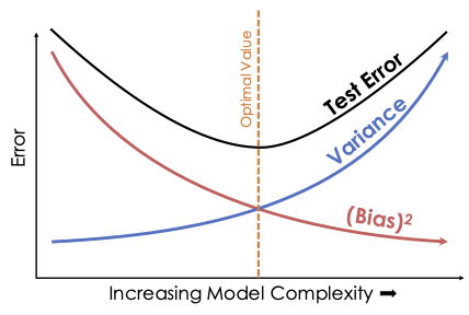
Fig. 16.4 Bias–variance trade-off#
Collecting more observations reduces bias if the model can fit the population process exactly. If the model is inherently incapable of modeling the population (as in our synthetic example), even infinite data cannot get rid of model bias. In terms of variance, collecting more data also reduces variance. One recent trend in data science is to select a model with low bias and high intrinsic variance (such as a neural network) but to collect many data points so that the model variance is low enough to make accurate predictions. While effective in practice, collecting enough data for these models tends to require large amounts of time and money.
Creating more features, whether useful or not, typically increases model variance. Models with many parameters have many possible combinations of parameters and therefore have higher variance than models with few parameters. On the other hand, adding a useful feature to the model, such as a quadratic feature when the underlying process is quadratic, reduces bias. But even adding a useless feature rarely increases bias.
Being aware of the bias–variance trade-off can help you do a better job fitting models. And using techniques like the train-test split, cross-validation, and regularization can ameliorate this issue.
Another part of modeling considers the variation in the fitted coefficients and curve. We might want to provide a confidence interval for a coefficient or a prediction band for a future observation. These intervals and bands give a sense of the accuracy of the fitted model. We discuss this notion next.